Lookup using INDEX () function and MATCH () function to lookup from the right hand side
Subject Line
You’re right about it; you can lookup values from the right side
Overview
Sometimes you may want to lookup value in a different way. There could be a table where you would want to use any column and then traverse from right to left to search according to the column. As you know the LOOKUP () function looks up values from left side and returns the value from the right hand side i.e. it works from left side of the table towards the right side of the table. What if you want to lookup value from the right side and return the value from the right side. You will need to use two functions which are INDEX () function and MATCH () function to get the desired result.
Working
Let’s understand the working with the help of an example.
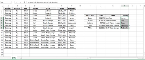
In the example used below Table 1: Sales of Desktops shows Sales of the Product (Laptop) by Year, Quarter, Country wise, Zone wise and Sales representative sales for their Zone.
Sales Representative is the last column in the table (Column G)
The management wants a report in the format (Sales Rep, Sales, Zone and Country) for only a few Sales Representatives. If you were to compare the report with the data the columns are in reverse order.
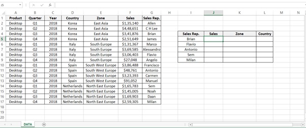
Table 1: Sales of Desktops
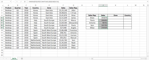
Step 1: We want Sales made by Brian so type the below formula (shown in cell J5)
=INDEX($F$2:$F$17,MATCH(I5,$G$2:$G$17,0))

INDEX function returns a value in a table based on the intersection of a row and column position within that table.
Syntax
=INDEX (array, row_num, [col_num], [area_num])
Arguments
· Array – A range of cells, or an array constant.
· row_num – The row position in the reference or array.
· col_num – [optional] The column position in the reference or array.
· area_num – [optional] The range in reference that should be used.
Match option is used to locate the position of a lookup value in a row, column, or table.
Sytax
=MATCH (lookup_value, lookup_array, [match_type])
Arguments
· lookup_value – The value to match in lookup_array.
· lookup_array – A range of cells or an array reference.
· match_type – [optional] 1 = exact or next smallest (default), 0 = exact match, -1 = exact or next largest.
Row_Num
![]()
=INDEX($F$2:$F$17,MATCH(I5,$G$2:$G$17,0))
![]()
Array
Step 2: Drag the formula for other sales representative. Select the cells and Press Ctrl+D.
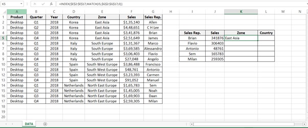
Step 3: We want Zone of Brian so type the below formula (shown in cell K5)
=INDEX($E$2:$E$17,MATCH(I5,$G$2:$G$17,0))
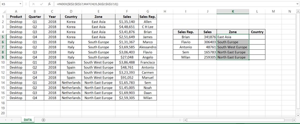
Step 4: Drag the formula for other sales representative to get their respective Zone. Select the cells and Press Ctrl+D
Step 5: Finally we want Country of Brian so type the below formula (shown in cell L5)
=INDEX($D$2:$D$17,MATCH(I5,$G$2:$G$17,0))

Step 6: Drag the formula for other sales representative to get their respective Country. Select the cells and Press Ctrl+D
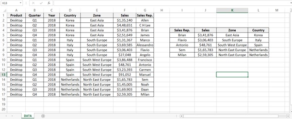
Step 7: Final result after formatting the currency to Dollars
Understanding how the formula works with the help of Evaluate Formula
Step 1: Select the cell (J5 in this case) that you want to evaluate. Only one cell can be evaluated at a time.
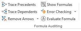
Step 2: On the Formulas tab click on Evaluate Formula in Formula Auditing group
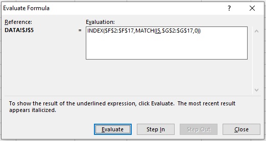
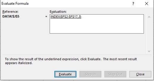
Step 3: Evaluate Formula dialog box will appear
Click on Evaluate
It check I5 Value
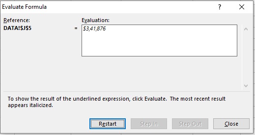
Step 4: Brian is the result

Step 5: Row no. is 3
Step 6: Result
Scope of Usage
ü Can be used to perform a vertical lookup by searching for a value
ü Can be used to lookup values from Right hand side of the table
ü Can be used in situations when you need to reverse your search operation
ü Can be used in combination of INDEX () function and MATCH () function