Career Growth

Excel Videos

Excel Blogs

Replace Blank Cells with Zeros in Excel Pivot Tables
August 15, 2022
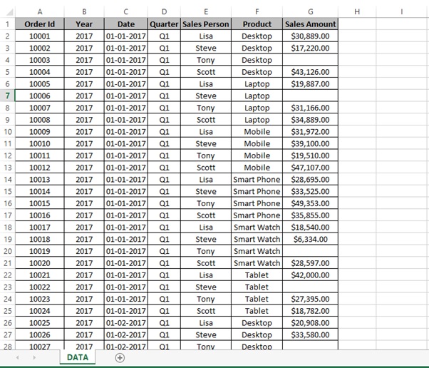
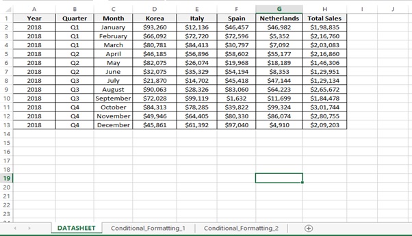
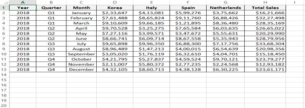
Sometimes you will have to prepare summary of the raw data which can have missing or blank values. Once you generate the Pivot table the values will be shown as blanks in the Pivot table also. To make the Pivot table presentable and uniform especially in case of numeric values you can replace the blank values with zeros. Also once you generate the Pivot Table you can identify the number of blanks in the data and you may want to replace the blank value with some value of your own. So your Pivot looks better
Find the 2nd,3rd,4th or Nth Value in excel
August 15, 2022
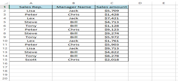
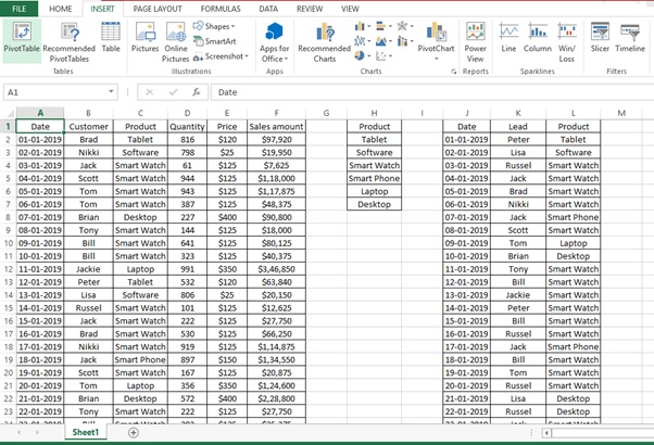
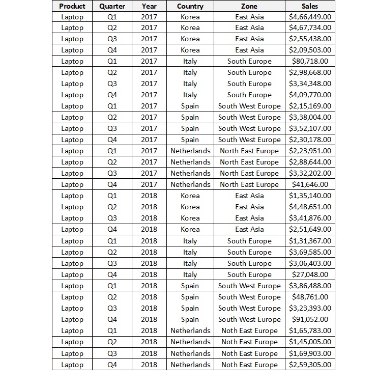
Sometimes you may need to look up the 2nd,3rd,4th or Nth value from a table i.e. based on the occurrences of the values dynamically lookup for the values. VLOOKUP () Function lookups a value from left side of the column and returns the first matching value based on column index number. We have to use the below formulas to get the desired result
Three way Lookup
August 15, 2022
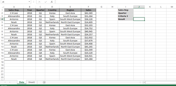
Sometimes you may want to do a three way lookup i.e. search on a combination of values in a table. You can build your own formula that to perform a Three -way lookup with help of INDEX and MATCH function. It can achieved with concatenating the Lookup value and use array formula to get the desired result.
Using Drop Down lists as Lookup Values
August 15, 2022
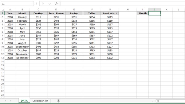
Sometimes you may want to look up a value in a table using both rows and columns. You can build your own formula that to perform a two-way lookup with help of INDEX and MATCH function. In this example we are using the row and column reference from drop down list.
Case Sensitive Lookup in Excel using Exact function
August 15, 2022
As you already know a usual VLOOKUP () formula is case sensitive and will ignore case. Sometimes you may want to lookup exact value in a table. Hence we use Exact () function along with INDEX & MATCH function with an array formula to retrieve the desired result from the table.
Combine VLOOKUP and CHOOSE with Multiple Criteria
August 15, 2022
Sometimes you may need to get the output without using helper column. What is a helper column? We create a separate column and concatenate both the values in a separate column and then use it as a lookup value to get the desired result. But in order to do this without a helper column, we will have to combine VLOOKUP function along with CHOOSE function to get the desired result.
Negative Positive icons using Conditional Formatting
August 15, 2022
Sometimes you may want to rate status reports based on different indicators just like the traffic lights using red, amber (yellow) and green to signify different scale ratings. There is always a need to make reports appealing based on the format and presentation. Conditional formatting is a feature of Excel which allows you to apply a format to a cell or a range of cells based on certain criteria provided by the user. Once the formatting is done it reflects the change in formatting if values are changed.
Linking a slicer to 2 Pivot tables from different data sources
August 15, 2022
Sometimes you may need to slice and dice or drill down for certain reports. Drill-down reports are used to validate and verify and also to zoom in to find particulars about a single value. Slicer is a powerful way to filter pivot table data. We can click on an item in a slicer to filter the data in the pivot table.Slicers provide buttons that you can click to filter tables or Pivot table. You can also link one slicer with 2 Pivot Tables based on a different data sources.
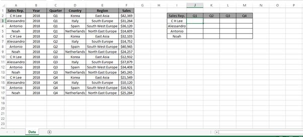
Create Multiple Pivot Tables with Show Report Filter Pages
August 15, 2022
As we know Pivot tables are used to Summarize, Sort, Reorganize, and Group, Count, Total or Average data. But sometimes we many need to make copies of the pivot table for each unique item in a field. This will help us to save lot of time with our everyday work as the pivot table can be created instantly Sometimes we need to make an exact copy of pivot table for each unique item in a field.
2 way lookup using INDEX(),MATCH(),MATCH() function.
August 15, 2022
Sometimes you may want to lookup a value in a table using both rows and columns. You can build your own formula that to perform a two-way lookup with help of INDEX and MATCH function.
Lookup using built in LOOKUP () function from right side
August 15, 2022
Sometimes you may want to lookup value in a different way. There could be a table where you would want to use any column and then traverse from right to left to search according to the column. As you know the LOOKUP () function looks up values from left side and returns the value from the right hand side i.e. it works from left side of the table towards the right side of the table. What if you want to lookup value from the right side and return the value from the right side.
How to pull values from Pivot Table using GETPIVOTDATA()
August 15, 2022
Sometimes the management may request for different set of reports summarized based on different conditions. You need not create a pivot table every time. With the help of GETPIVOTDATA we can extract correct data from the Pivot table even if the pivot table layout is changed as it uses criteria to lookup.
Lookup up from multiple tables using IF statement
August 15, 2022
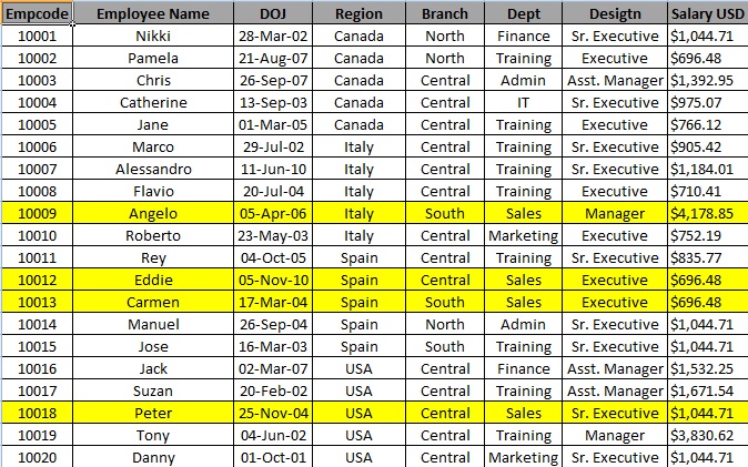
Sometimes you may need to look up data or values from multiple tables on the basis of some conditions using IF statements which are incredibly robust. In this case we use Vlookup along with IF statement to search the value as per your criteria. There could be possibilities of the conditions being recorded separately also; so the lookup criteria which would make your search operation slightly complex. Therefore, in order to simplify the search operation you can combine the ranges you wish to use for your conditions but only in case where you need to make logical comparison using minimal conditions you can make use of Vlookup along with IF statement.
Calculated values in Pivot Table
August 15, 2022
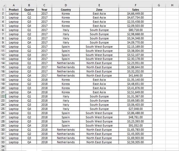
Would you want to learn about how to create summarized information in excel. You can create a Pivot Table in excel and create your own calculated field to perform analysis on the pivot table. You can also use the calculated fields to perform further calculations or analysis. If you not aware then, Pivot tables are used to Summarize, Sort, Reorganize, and Group, Count, Total or Average data.
Multiple Chained Lookup
August 15, 2022
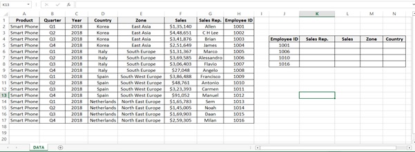
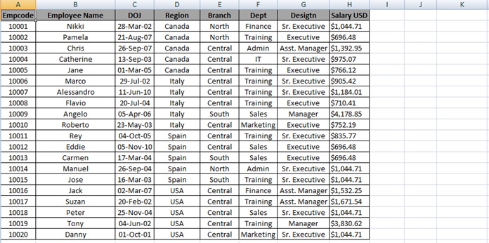
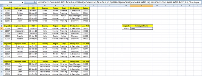
You can make use of VLOOKUP () function and then nest or chain the function for each table. If there are 4 tables then you will make use of four VLOOKUP () functions in the same formula. We have four tables in our example for employee information. Hope you know that to write a formula in excel you can use = sign on a cell.

Topics covered in Excel School
Designed for modern Excel
Excel School is designed for modern Excel – Excel 2019, Excel 2016, Office 365. While you can practice the concepts in older versions of Excel, to get the most out of it, use latest version of Excel or Office 365.

Getting Started

Intro to Excel
Setting up tables
Cleaning bad data
Cleaning using Power Query
Writing formulas
Creating pivot tables
Making charts
Filtering & sorting
Shortcuts
Data + Tables + PQ

Excel Tables
Filtering, slicing tables
Bad data to good with PQ
Unpivoting data with PQ
Merging multiple files to one table
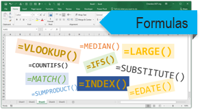
Writing Formulas

Referencing data
IF condition, CHOOSE, IFS
Statistical analysis
Conditional sum, count
Lookups
Advanced Lookups
Date formulas
Text analysis
Sentiment analysis
Exploratory data analysis
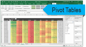
Making Pivot Tables

Creating pivot tables Data model + relationships Multiple table pivots Customizing pivots Extra calculations in Pivots Grouping data Slicing and dicing GETPIVOTDATA

         Adv. Pivot Table bonus
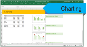
Charts + Graphs

Intro to Charting
Picking right charts
Anatomy of Excel chart
Formatting charts
New charts in Excel 2016
Budget vs. Actual charts
Then vs. Now charts
Conditional charts
Sparklines
Interactive charts

Advanced Concepts

Data validation
Creating templates
Workbook protection
Publishing to web
Shapes + pictures
Navigation buttons
Priting
Form controls
Custom ribbons

Optional module on

Dashboards

What is a dashboard?
Process for dashboards
Business dashboard #1
Business dashboard #2
Business dashboard #3
Employee Dashboard
Financial metrics dashboard
KPI Dashboard
Web enabled dashboard
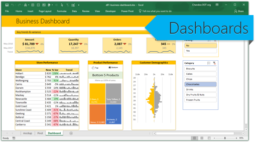
Excel Dashboards

Dashboards from Excel School

Previous
Next

FAQ

Most frequent questions and answers

In Excel School we are using Excel 2016 / 2019 / Office 365. While you can apply the concepts to older versions of Excel (Excel 2013, 2010 or 2007), to get the most out of it, use Excel 2019, 2016 or Office 365.

Yes. You get 25% discount when purchasing 3 or more memberships for Excel School programs.

If you want to enroll a large team (50 or more people), please email chandoo.d@gmail.com

Power Query:

Power Query is a data management interface for Excel (and Power BI). Using Power Query you can connect to any kind of data sources (SQL Databases, workbooks, online data sets, web pages etc.) and bring the data to Excel (or Power BI). Power Query also lets you manipulate data by adding columns, changing shape of the data or combining data sets. It is part of Excel functionality in 2016 or Office 365 versions. For older versions, you can download the free add-in from Microsoft website.

Power Pivot:

Power Pivot is a calculation engine for pivot tables in Excel (and Power BI). Using Power Pivot you can enhance your pivot tables and add extra calculations easily. Power Pivot is available by default in Excel 2016, Office 365 and Excel 2013. For other versions of Excel, you can download the free Power Pivot add-in from Microsoft Website

You may. Excel School is recorded on Excel 2016 / O365 for Windows. Most of the formulas, charts & techniques work equally well on Mac. I suggest borrowing a PC for practicing other ideas.

Yes you can. After your payment you will get it automatically.

If you need it in a specific format, please email chandoo.d@gmail.com with “invoice” in the subject. 

We can also invoice you before purchase so you can make a payment against it. Please email.

Yes. Excel School is a one time payment program. There are no recurring charges.

No problem. Just email me at chandoo.d@gmail.com or call me on +64 21 070 1136 so I can help you make a decision

Thank you...

I am thankful to all the readers and supporters of Chandoo.org. Thank you for considering my Excel School program. I am excited to share this powerful course with you so that you can be awesome at what you do. Thank you. 🙏

PS: As of writing this, more than 1,200 students have already enrolled in Excel School 2.0. Don’t miss out the chance to learn and use powerful features of Excel.

Your Cart

Job Maverick

Total

147.00 USD

Proceed To Pay