How to Create Pivot Table and Pivot Chart using VBA
AS-IS Scenario
Mr. Andre Dell (MIS Executive) has to prepare a sales report which involves Pivot table and Pivot chart (Bar Chart) to be created from the sales data which represents Sales done as per Region and Order Date. He has to prepare this report and send to his manager on weekly basis.
TO-BE Scenario
It takes little time to prepare this report but he decides to take the help of macro to automate this process.
Let’s go through the Sales Data before we automate the report.
We have 16 Columns in the Sales_Raw_Data.xlsx i.e. Order ID, Order Date, Customer ID, Customer Name, Sales Rep. Name, City, State, Country, Postal Code, Market, Region, Mobile No., Product, Price, Quantity and Sales Amount.
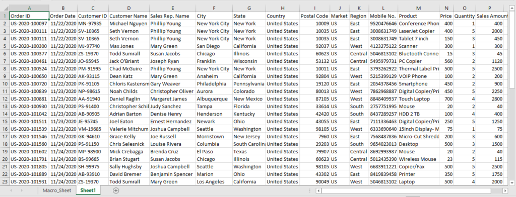
We have to Copy the Data from Sales_Raw_Data.xlsx to Sales_Data.xlsm in Sheet1.
Let’s follow the below steps to Create Pivot Table.
Step 1. Open Sales_Raw_Data.xlsx (contains Raw Data) excel file.
Step 2. Open Sales_Data.xlsm (contains Code) excel file.
Step 3. Press Alt+F11
Step 4. Go to Insert Menu
Step 5. Select Module
Step 6. Module will be inserted
Step 7. Select Module 1
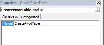
Step 8. Go to Properties Window
Step 9. Change the name to CreatePivotTable in (name)
Step 10. Go to Code Window and type the below code.
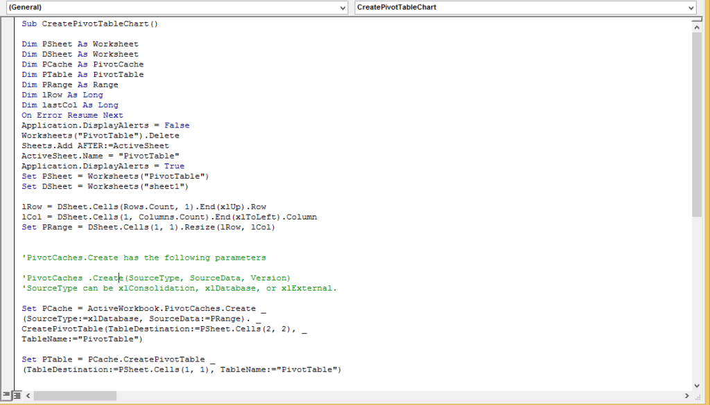
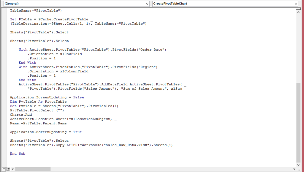
Sub CreatePivotTable()
Dim Wk As Workbook
Dim PSheet As Worksheet
Dim DSheet As Worksheet
Dim PCache As PivotCache
Dim PTable As pivottable
Dim PRange As Range
Dim LastRow As Long
Dim LastCol As Long
On Error Resume Next
Application.DisplayAlerts = False
Workbooks(“Sales_Raw_Data”).Activate
Worksheets(“Total_Sales”).Delete
Sheets.Add Before:=ActiveSheet
ActiveSheet.Name = “Total_Sales”
Application.DisplayAlerts = True
Set PSheet = Workbooks(“Sales_Raw_Data”).Worksheets(“Total_Sales”)
Set DSheet = Workbooks(“Sales_Raw_Data”).Worksheets(“Sales_Data”)
LastRow = DSheet.Cells(Rows.Count, 1).End(xlUp).Row
LastCol = DSheet.Cells(1, Columns.Count).End(xlToLeft).Column
Set PRange = DSheet.Cells(1, 1).Resize(LastRow, LastCol)
Set PCache = ActiveWorkbook.PivotCaches.Create _
(SourceType:=xlDatabase, SourceData:=PRange). _
CreatePivotTable(TableDestination:=PSheet.Cells(2, 2), _
TableName:=”Total_Sales”)
Set PTable = PCache.CreatePivotTable _
(TableDestination:=PSheet.Cells(1, 1), TableName:=”Total_Sales”)
Sheets(“Total_Sales”).Select
With ActiveSheet.PivotTables(“Total_Sales”).PivotFields(“Order Date”)
.Orientation = xlRowField
.Position = 1
End With
With ActiveSheet.PivotTables(“Total_Sales”).PivotFields(“Region”)
.Orientation = xlColumnField
.Position = 1
End With
ActiveSheet.PivotTables(“Total_Sales”).AddDataField ActiveSheet.PivotTables( _
“Total_Sales”).PivotFields(“Sales Amount”), “Sum of amount”, xlSum
With ActiveSheet.PivotTables(“Total_Sales”).PivotFields(“State”)
.Orientation = xlPageField
.Position = 1
End With
Application.ScreenUpdating = False
Dim PvtTable As pivottable
Set PvtTable = Sheets(“Total_Sales”).PivotTables(1)
PvtTable.PivotSelect (“”)
Charts.Add
ActiveChart.Location Where:=xlLocationAsObject, _
Name:=PvtTable.Parent.Name
Application.ScreenUpdating = True
End Sub
Step 11. Go to Macro_Sheet in the Sales_Data.xlsm excel file
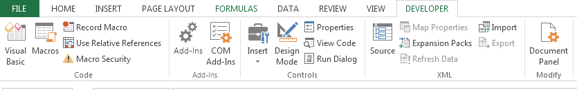
Step 12. Go to Developer Tab
Step 13. Go to Insert in Controls Section
Step 14. Select Button (Form Control)
Step 15. Place the Button inside the excel sheet.
Step 16. Right click on the Button and select Edit Text
Step 17. Change the Text to Create Pivot Table & Pivot Chart
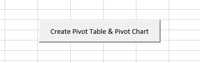
Step 18. Right Click on the Button
Step 19. Select Assign Macro and Select CreatePivotTable
Step 20. Click on Create Pivot Table & Pivot Chart Button to run the Macro.
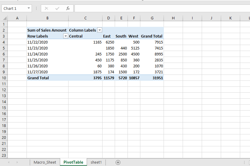
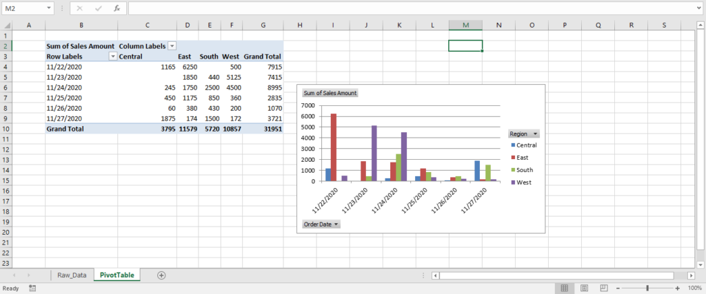
Step 21. First Pivot Table is created by inserting a Sheet with PivotTable as name of the sheet
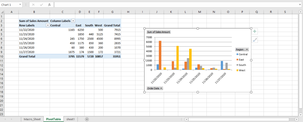
Step 22. Then Pivot Chart is created on the same sheet(PivotTable).
Step 23. A copy of PivotTable is created and moved after Raw_Data sheet in the Sales_Raw_Data.xlsx excel files.
By this way Mr. Andre Dell has automated the task of creating Pivot Table and Pivot Chart.