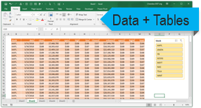
Working

Let’s understand with the working help of the example below (Table1: Sales Report)

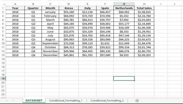
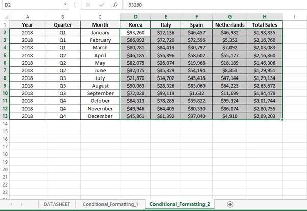
Table 1: Sales Report

We have 2 Tab’s for conditional formatting i.e. Conditional_Formatting_1 & Conditional_Formatting_2

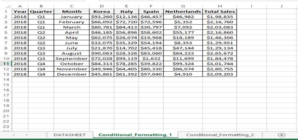
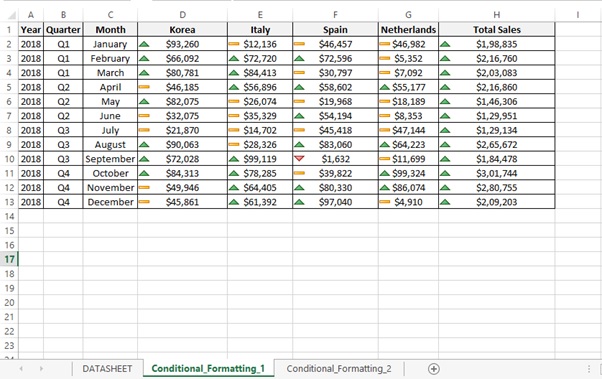
Figure 1.1 Conditional_Formatting_1

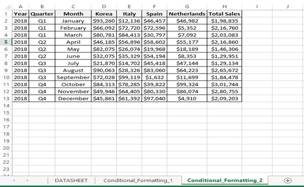
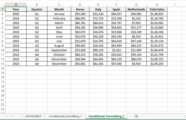
Figure 1.2 Conditional_Formatting_2

Let’s apply conditional formatting on the below table (Conditional_Formatting_1 tab)

Step 1: Select the data(D2:H13)

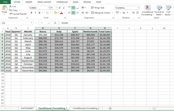
Step 2: Go to Home tab

Step 3:  Click on Conditional Formatting in the Styles group

Step 4: Click on New Rule

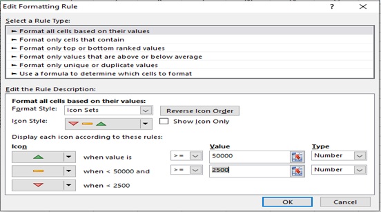
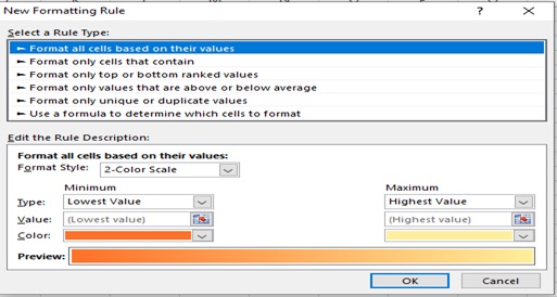
Step 5: Select Format all cells based on their values

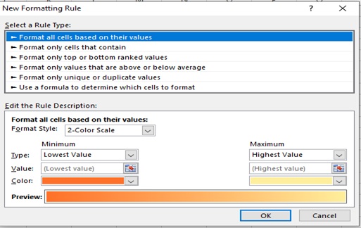
Step 6: Select Icon Sets from Format Style and select Icon Style

Step 7: Select the Type as number and enter the value as mentioned in the image.

Step 8: Based on the criteria we get the below results.

Let’s apply conditional formatting on the below table (Conditional_Formatting_2 tab)

Step 1: Select the data(D2:H13)

Step 2:  Go to Home tab

Step 3: Click on Conditional Formatting in the Styles group

Step 4: Click on New Rule

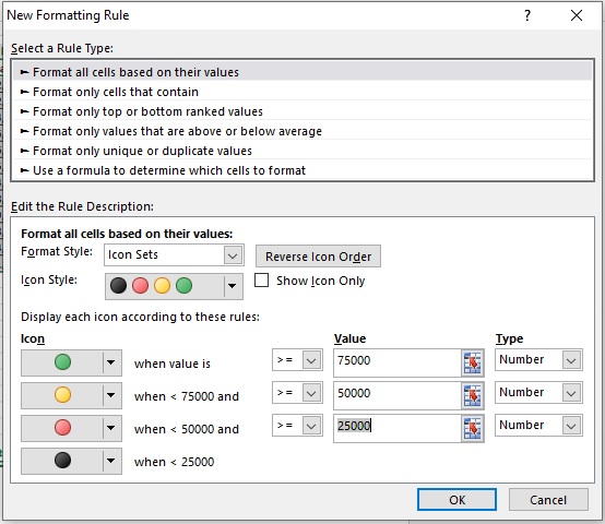
Step 5: Select Format all cells based on their values

Step 6: Select Icon Sets from Format Style and select Icon Style

Step 7: Select the Type as number and enter the value as mentioned in the image.

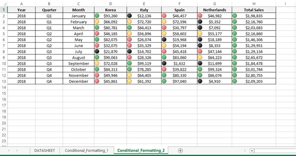
Step 8: Based on the criteria we get the below results.

Scope of Usage

ü  Can be use for management reporting

ü  Can be used to add visual appeal to reports

ü  Can be used to highlight cells in a table

ü  Can be used to choose and apply selected colour

ü  Can be used to use icon styles

ü  Can be used to use format styles

ü  Can be used to define rules or criteria