Working

Let’s understand with an example of Sales table.

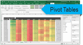
We have a report (Figure1: Sales by Sales Person for the year 2017 and 2018)

As you can see some of the values are blanks in Column G which is the Sales amount.

You have to create a summary of quarterly Sales made by Sales Peron for the year 2017 and 2018.

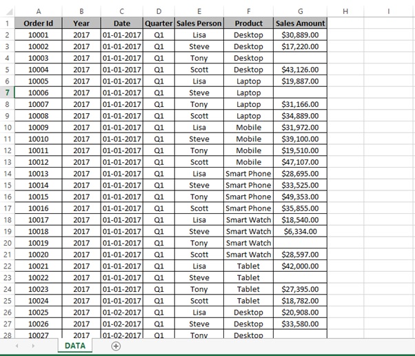
Figure1: Sales by Sales Person for the year 2017 and 2018

Step 1: Let’s begin with by creating Pivot table.

Select the table range.

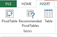
Step 2: Click on INSERT Tab

Step 3: Click on PivotTable Option in the Tables group

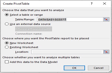
Step 4: Create PivotTable dialog box will appear

Step 5: Click on OK

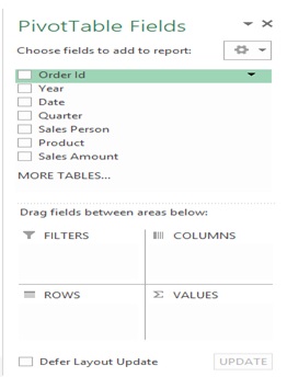
Step 6: PivotTable Fields will be appear in the new sheet

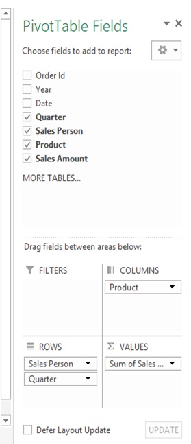
Step 7: Drag the Sales Amount field in VALUES area.

Step 8: Drag the Product to COLUMNS area.

Step 9: Drag the Sales Person & Quarter to ROWS area

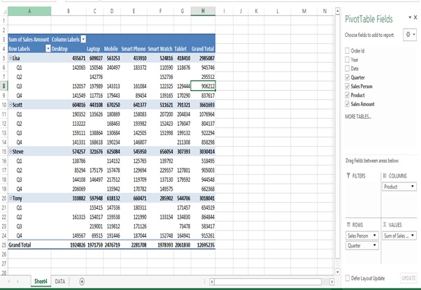
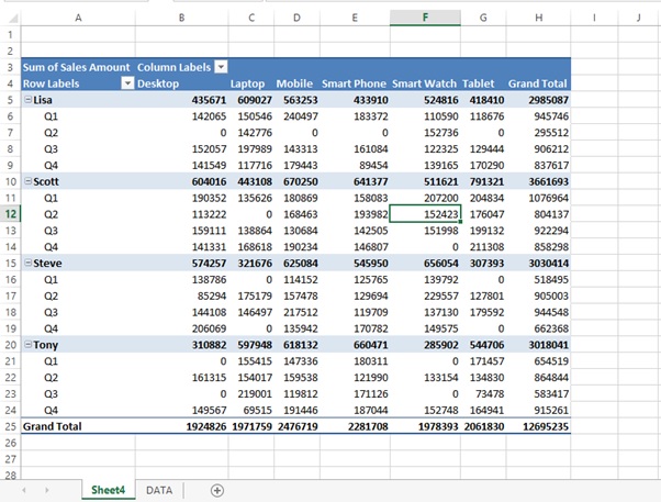
Step 10: You can see the below summary after dragging the field to their respective area.

Step 11: You can see that there is blank in some fields in the below figure.

Step 12: Click on any cell inside the Pivot Table.

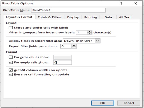
Step 13: Click on PivotTable Options…

Step 14: PivotTable Options dialog box will appear

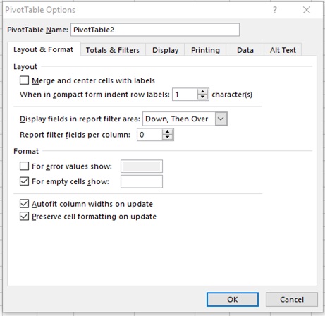
Step 15: Type 0 in the “For empty cells show” in the Format section in the Layout & Format tab.

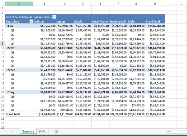
Step 16: You can see the value of 0 in place of the missing fields in the PivotTable.

Step 17: Click on any cell inside the Pivot Table

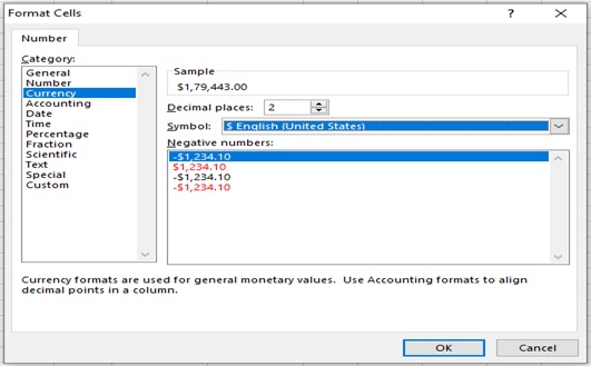
Step 18: Click on Number Format

Step 19: Select $ English (United States) from the Symbol as shown in the below figure

Step 20: Final result

Scope of usage

ü  Can be used to provide your own value to fill missing values in the Pivot Table

ü  Can be used to prepare uniform and meaningful summaries

Can be used to replace blank cells in the Pivot Table55