Multiple Chained Lookup

Overview

You can make use of VLOOKUP () function and then nest or chain the function for each table. If there are 4 tables then you will make use of four VLOOKUP () functions in the same formula. We have four tables in our example for employee information. Hope you know that to write a formula in excel you can use = sign on a cell.

Working

Lets understand the working of VLOOKUP () function

1.       The value you want to look up which is called the lookup value 

2.       The range where the lookup value is located

Note: the lookup value should always be in the first column in the range for VLOOKUP to work correctly. For example, if your lookup value is in cell C2 then your range should start with C.

3.       The column number in the range that contains the return value. For example, if you specify B2:D11 as the range, you should count B as the first column, C as the second, and so on.

Optionally, you can specify TRUE if you want an approximate match or FALSE if you want an exact match of the return value. If you don’t specify anything, the default value will always be TRUE or approximate match. You can also use 1 or 0

IFERROR () Function

IFERRROR () function is used along with the VLOOKUP () function in so that if the value is not found you can catch the #N/A error and replace it with you own message

Nesting

You can nest VLOOKUP () function inside the IFERRROR () function

By nesting multiple VLOOKUPs inside the IFERROR function, the formula allows for sequential lookups. If the first VLOOKUP fails, IFERROR catches the error and runs another VLOOKUP. If the second VLOOKUP fails, IFERROR catches the error and runs another VLOOKUP, and so on.

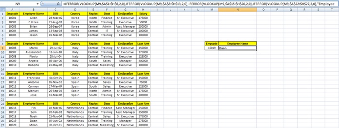
The example used is as below

The Formula is constructed as below

=IFERROR(VLOOKUP(M9$A$1:$H$6,2,0),IFERROR(VLOOKUP(M9,$A$8:$H$13,2,0),IFERROR(VLOOKUP(M9,$A$15:$H$20,2,0),IFERROR(VLOOKUP(M9,$A$22:$H$27,2,0),”Employee not found”))))

Enter the employee code in the cell M9. If the employee code exists it will return the Employee Name else it will return the message “Employee not found”

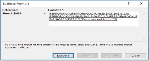
Understanding how the formula works with the help of Evaluate Formula

Step 1: Select the cell (M9 in this case) that you want to evaluate. Only one cell can be evaluated at a time.

Step 2: On the Formulas tab click on Evaluate Formula in Formula Auditing group

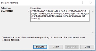
Step 3: Evaluate Formula dialog box will appear.

Step 4: Click Evaluate to examine the value of the underlined reference. The result of the evaluation is shown in italics.

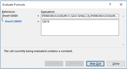
If the underlined part of the formula is a reference to another formula, click Step In to display the other formula in the Evaluation box. Click Step Out to go back to the previous cell and formula.

Step 5: After clicking on Step In button we get the lookup value.

Step 6: Click on Step Out

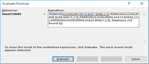
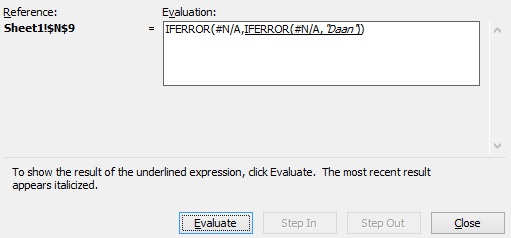
Step 7: Click on Evaluate

Step 8: Formula (VLOOKUP) gets executed.

Step 9: #N/A appears as result

Step 10: Repeat the steps till the last VLOOKUP result

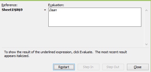
Step 11: Final result

Step 12: Click on Close

ü  Can be used to specify your own output message in case of values not found

ü  Can be used with multiple tables of data

ü  Can be used to nest several LOOKUP () functions

ü  Can be used for sequential lookups

ü  Can be used for a single branch of information

ü  Can be used to make short formula